Robustness
pyAMNESIA aims at analyzing many calcium images to produce statistics. Among all the criteria that could quantify its relevancy, the most important is without any doubt:
Important
Does pyAMNESIA perform great on all calcium imaging sequences?
The following sections explain how one can get the best result possible while using the tool.
Parameter tuning
In order for you to choose the best set of parameters for each analysis scenario, we provide in this documentation a description of every tunable parameter of the tool. To read these descriptions, please see the Parameter selection section of the OVERVIEW page that corresponds to the analysis you are running.
These descriptions can also be found in CICADA, when clicking on the ? icons.
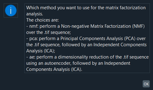
A help window in CICADA.
We also provide some configuration templates that you can use for your analysis.
Consecutive clusterings
There are different scales of components, that we could mistakenly call micro, meso and macroscopic.
- microscopic: a pixel;
- mesoscopic: a neurite, a morphological branch;
- macroscopic: a set of several branches, the whole sequence.
The clustering algorithm finds groups of coactive components.
When the projection_method parameter is set to 'pixel', the algorithm forms groups of pixels, and thus forms mesoscopic components from microscopic components.
When the projection_method parameter is set to 'branch', the algorithm forms groups of branches, and thus forms macroscopic components from mesoscopic components.
In the willingness to compare both methods, we developed a functionality of consecutive clusterings. It allows the tool to run several clusterings in a row, every time increasing the clusters scale. It simply works by taking the average trace of each cluster, and considering the clusters as input components of the next clustering.
In the CLI and the GUI, we only need to pass the Clustering_*/ folder as an input to the clustering module.
Warning
As the current module folder is created before opening the file dialog box, you must select the penultimate Clustering_*/ folder, the last one being empty at this time.
Note
Depending on the scale, you are expected to change the t-SNE and HDBSCAN parameters values from one clustering to another.
For example, if your first clustering concerns skeleton pixels, you might want to find mesoscopic clusters, of a dozen of pixels. Then for your second clustering, you might want to find macroscopic clusters. The t-SNE and HDBSCAN parameters will then be expected to be lower (cf Clustering parameter selection).
Here is an example of 3 consecutive clusterings:
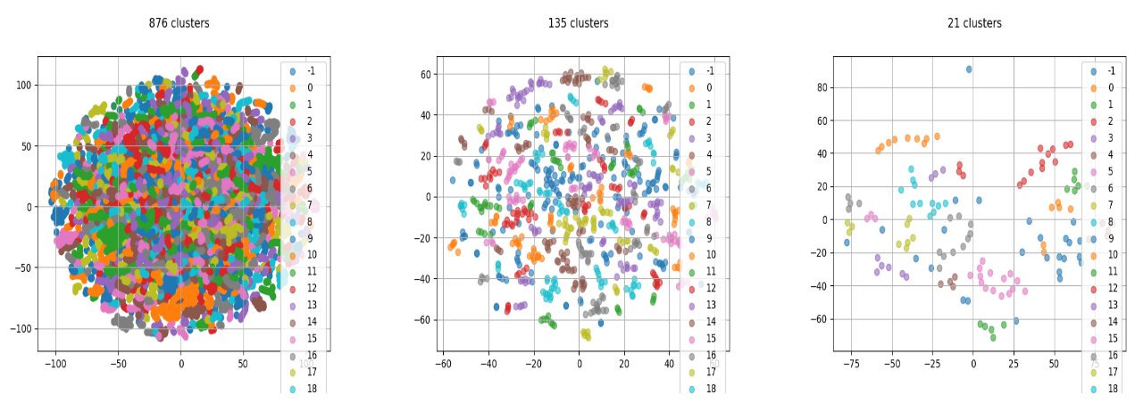
Consecutive clusters: from microscopic to macroscopic. Top: The 2D projected traces. Bottom: A cluster overlay (purple) on the skeleton (green).
Skip skeletonization
There are some sequences that cannot be well processed by the tool. For instance:
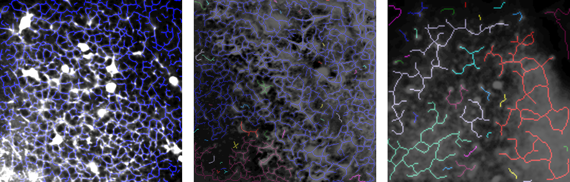
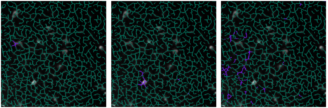
Some skeletonization results.
- The image at the left comes from a sequence that is quite optimal and therefore has been well-skeletonized.
- The sequence from which the image in the middle comes presents some flickering and has a lower resolution; yet its skeletonization is good.
- The image at the right, however, has a resolution that is too low. The tool has trouble determining the morphological structure of the data and thus produces an irrelevant skeletonization.
From this and other experiments, we can extract two main cases that could cause a bad skeletonization:
- a flickering of the sequence;
- a low resolution of the sequence.
In any of these cases, you can skip the skeletonization, directly performing a clustering or a matrix factorization.
Warning
This may increase the computational time of the analysis, as the skeletonization module also conducts a dimensionality reduction of the input data.
Note
Actually, we do not “skip” the skeletonization module. For computational reasons, we decide to keep the beginning of the Image skeletonization pipeline, only skipping the two last steps (skeletonization and skeleton cleaning). This allows to extract the binary image that represents the pixels that are active during the movie. As a consequence, the background and noise pixels are removed from the components to analyze, which reduces the dimension.
In order to do so, we set the projection_substructure parameter to 'active' (cf Skeleton parameter selection).
A movie projected on the active pixels.
The results are in the Skeleton_*/ folder, in the same format as when we don’t “skip” the skeletonization. Then, they can be used by the clustering or the factorization module.
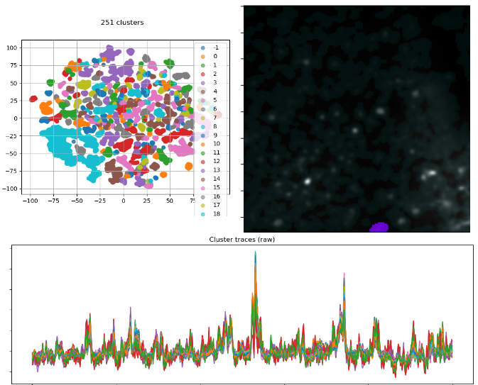
Results of clustering on the active sequence. Left: The 2D projected traces. Right: A cluster overlay (purple) on the summary image. Bottom: The traces of the pixels belonging to the overlaid cluster.
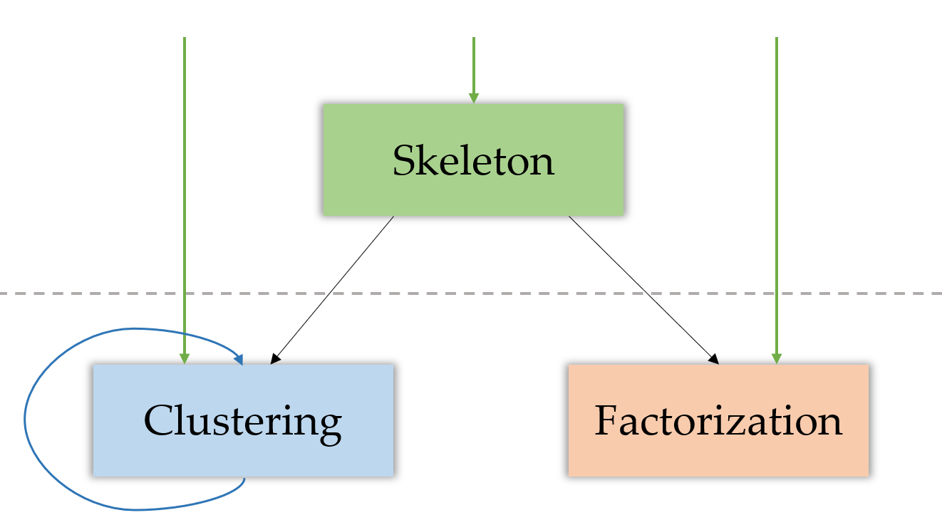
Finally, here is the structure of the approach, including the optional consecutive clusterings and skipping of skeletonization.