Factorization
Table of contents
In the next sections, the method illustrations (results, inputs…) focus on our study on calcium imaging data from the mice hippocampus (see Motivation for more info).
Methods
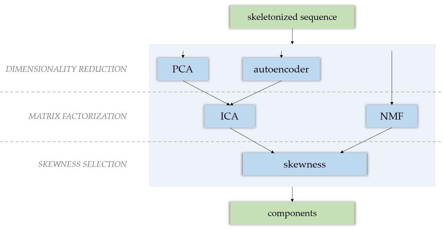
The factorization module provides several matrix factorization techniques to produce independent components from a .tif sequence, such as PCA (Principal Components Analysis), ICA (Independent Components Analysis) and NMF (Nonnegative Matrix Factorization). If you choose to perform an ICA, a dimensionality reduction is needed. For this, you can either perform a PCA, or use an autoencoder. After either a NMF or a PCA-ICA, components are selected by their skewness.
Let’s consider a .tif sequence matrix, of shape \((T, N_x, N_y)\), that is flattened into a matrix \(M\) of shape \((T, N_x\times N_y)\). Let’s note \(N:=N_x \times N_y\). This matrix can be the raw calcium imaging .tif sequence, or an output of the skeletonization module.
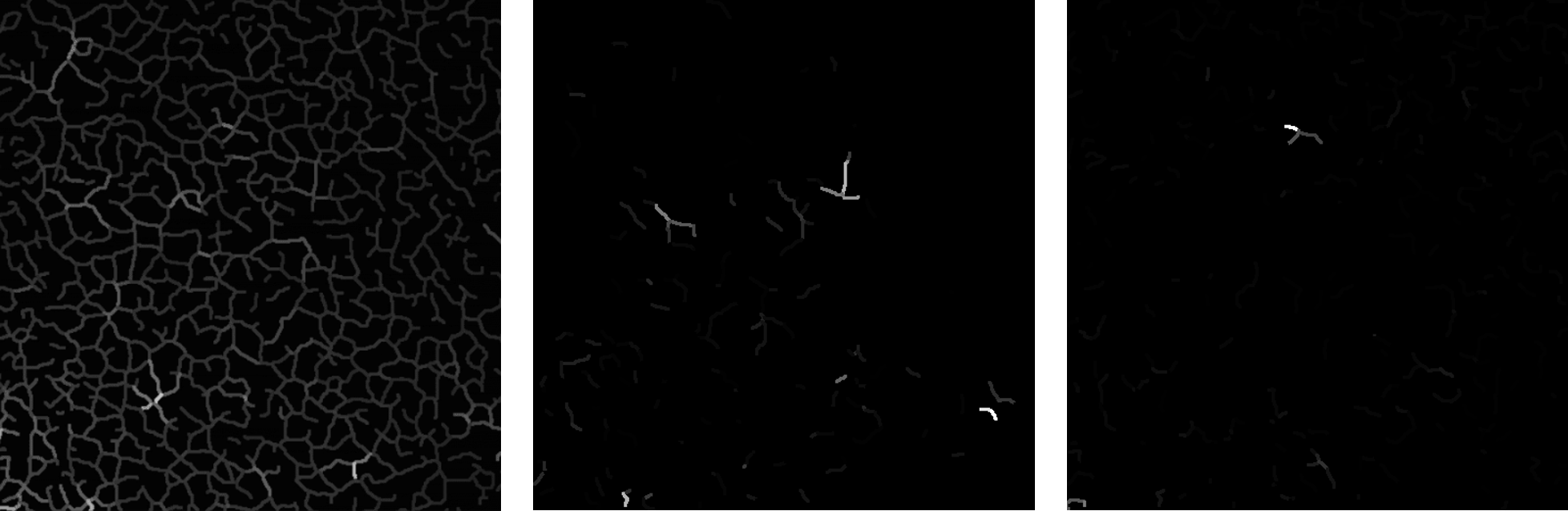
From left to right: a frame of the input skeletonized sequence; a component; another component.
Dimensionality reduction
The goal of dimensionality reduction here is to transform the \((T, N)\) matrix into a \((T_1, N)\) matrix, with \(T_1 \ll T\).
PCA
PCA (Principal Components Analysis) is a dimensionality reduction technique that analyses the \(p\)-dimensional points cloud data and finds the axis along which the variance is the highest, keeping them over the ones with a low variance. By omitting the axis with a low variance, we lose an equally small amount of information.
Theory
We want to find the vector \(u\) with the highest variance. Let’s project our data matrix \(A\) onto this vector:
The empirical variance \(v\) of \(\pi_u(A)\) is \(\frac{1}{K} \pi_u(M)^T\pi_u(M)\) (\(K\) being the number of pixels in \(A\)), and the covariance matrix \(\text{Cov}(A)\) is \(\frac{1}{K}A^TA\). We then have:
with \(\Delta=\begin{pmatrix}\lambda_1 & & \\&\ddots & \\& &\lambda_K\end{pmatrix}\), matrix of the eigenvalues of \(\text{Cov}(A)\).
We can then easily verify that \(v\) is then maximum when \(\tilde u\) is an eigenvector of \(\text{Cov}(A)\). In this case, we also have \(v=\lambda_i\), which means that the variance ratio is the same as the eigenvalues ratio.
Thus, to get the axis of our newly created space, we sort the eigenvalues and successively take them one after another, starting from the highest one, until we reached a sufficient amount of variance.
We uses the sklearn implementation of PCA in our tool. It features the necessary pre-processing (data centering).
Note
In our tool, we apply PCA to \(M^T\) for the sake of simplicity. It doesn’t change anything, except the computation time.
Indeed, PCA needs to compute the covariance matrix of the data, which is \(\text{Cov}(A)=A^TA\), of dimensions \((p,p)\) if \(A\) is of shape \((n,p)\). This computational time increases with \(p\).
Autoencoder
Warning
This functionality hasn’t been implemented yet.
Autoencoding is a machine learning self-supervised learning technique, which can be used as an alternative to PCA in the context of dimensionality reduction. An autoencoder is a neural network composed of an encoder and a decoder, that can be trained to encode (project the data to a lower dimensional latent space) then reconstruct the data as precisely as possible.
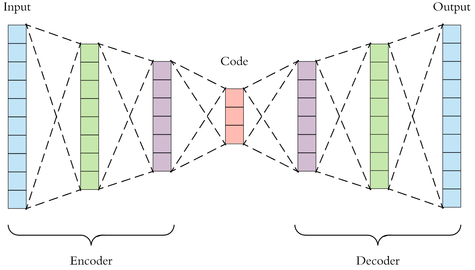
In the context of dimensionality reduction, what is important is the encoding operation.
The interest of using an autoencoder rather than a PCA is that is is more powerful and can perform more complex operations to encode the data. A linear autoencoder that has 3 layers (encoding, hidden and decoding) with linear activations will simply simulate a PCA; but replacing the linear activations by sigmoids or ReLUs allows the model to perform non-linear transformations of the data.
For more information on autoencoders, see [1]; for more information on the difference between PCA and autoencoders, see [2].
Source separation
ICA
The goal of ICA (Independent Components Analysis) is to separate a multivariate signal into additive subcomponents, assuming they are statistically independent from each other. It requires a dimensionality reduction as a pre-processing: PCA, or autoencoder. Thus, we want to reduce the \((T, N)\) once more, transforming the temporally reduced \((T_1, N)\) shaped matrix into a \((T_2, N)\) shaped matrix, with \(T_2 \ll T_1\).
To do so, ICA finds the independent components by maximizing their statistical independence (e.g. their non-gaussianity) [3].
We use the sklearn implementation of FastICA in our tool. It features the necessary pre-processing (whitening).

Some ICA components.
Warning
Our implementation of ICA may have some flaws and shouldn’t be taken as reference. It is adapted to pyAMNESIA and works well in this context but may have trouble to generalize.
NMF
The goal of NMF (Nonnegative Matrix Factorization) is to factorize a matrix \(V\) into two matrices \(H\) and \(W\), with \(V\approx H\times W\) and \(W,H\geq 0\). The interest of NMF here is that as since \(W\) is nonnegative, its columns can be interpreted as images (the components), and \(H\) tells us how to sum up the components in order to reconstruct an approximation to a given frame of the .tif sequence. One matrix approximates the elements of \(V\), the other infers some latent structure in the data. Moreover, as said in [4]:
As the weights in the linear combinations are nonnegative (\(H \geq 0\)), these basis images can only be summed up to reconstruct each original image. Moreover, the large number of images in the dataset must be reconstructed approximately with only a few basis images, hence the latter should be localized features (hence sparse) found simultaneously in several images.
We use the sklearn implementation of NMF in our tool.

Some NMF components.
Warning
As the components are not orthogonal, some superpositions happen: many pixels belong to several components.
Skewness selection
Once we have the components given by the methods described above, we can study their skewness, which is a measure of the asymmetry of the probability distribution of a real-valued random variable around its mean. Skewness is useful in two ways:
- As a factorization technique such as ICA leaves an ambiguity regarding the sign of the components [3], we want to be sure that all of them have the same orientation - a lot of dark pixels and some groups of bright ones. By studying the skewness of each component (i.e. of the repartition of the pixel values), one can identify the negative-skewed components and invert them.
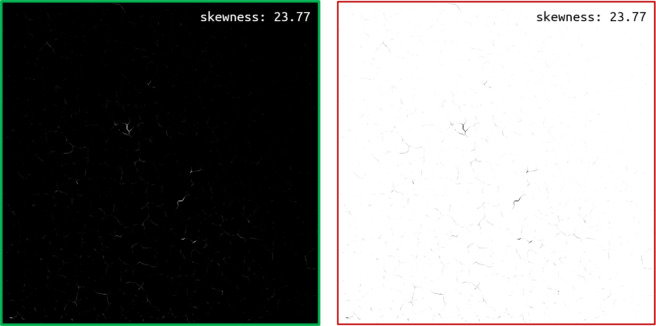
An image and its inverted image, with their respective skewness.
- Among these processed components, some may be noise. To remove these components that do not reflect the latent structure of the
.tifsequence, we can study their skewness. A skewness that is close to 0 means that the pixel intensity repartition is gaussian over the component, and that it is noise. We consequently introduce askewness_threshold, removing every component that do not pass this threshold.By looking at the skewness distribution histogram of the components, one can see that there is a peak of low-skewed components near 0. Very often, setting theskewness_thresholdto0.1is a good choice.
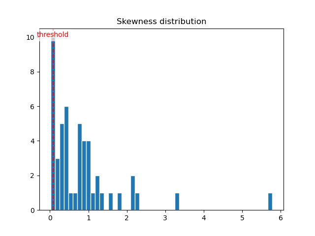
Components skewness distribution histogram.
Clipping
Among the final components, some may have some negative pixels. As we want to obtain components that can be interpreted as images (i.e. nonnegative matrices), we could try clipping them by setting to 0 the negative pixels:
Note
As the outputs of NMF are already positive, clipping is not necessary after a NMF.
Even if there is no mathematical justification to this operation, we observe that a PCA followed by an ICA and a clipping gives nearly the same results as a NMF. We thus chose to keep this operation in our tool.

Left: a NMF component; Right: the same component, obtained by PCA, ICA and clipping (better zoomed).
Parameter selection
Selecting factorization_method
- type:
str - default:
'nmf'
The factorization_method parameter selects which method is going to be used for the matrix factorization analysis. The choices are:
'nmf': perform a Non-negative Matrix Factorization (NMF) over the.tifsequence.
Note
When factorization_method is set to 'nmf', element_normalization_method must be set to None to make sure the input matrix is nonnegative.
'pca': perform a Principal Components Analysis (PCA) over the.tifsequence, followed by an Independent Components Analysis (ICA);'ae': perform a dimensionality reduction of the.tifsequence using an autoencoder, followed by an Independent Components Analysis (ICA).
Selecting nb_comp_intermed
- type:
int - default:
100
When choosing the 'ae' or 'pca' factorization method, you ask pyAMNESIA to perform a dimensionality reduction and then a source separation. The intermediate number of components specifies the number of dimensions you want the output of the dimensionality reduction to have.
The dimensionality reduction can be seen as an operation that has the signature f : (nb_frames, nb_pixels) -> (nb_comp, nb_pixels).
Selecting nb_comp_final
- type:
int - default:
50
This parameter specifies the number of components you want in the final output. If 'ae' or 'pca' is chosen for factorization_method, it has to be less than nb_comp_intermed and will be set to nb_comp_intermed if it is not.
Selecting skewness_threshold
- type:
float - default:
0.08
After having computed the final components, you can ask pyAMNESIA to check their skewness (measure of gaussianity). If the skewness of a component is too low, it means that it is noise and we remove it. All components of skewness inferior to skewness_threshold will be removed after the factorization.
| [1] | Building Autoencoders in Keras, The Keras Blog, https://blog.keras.io/building-autoencoders-in-keras.html |
| [2] | PCA & Autoencoders: Algorithms Everyone Can Understand, Thomas Ciha, https://towardsdatascience.com/understanding-pca-autoencoders-algorithms-everyone-can-understand-28ee89b570e2 |
| [3] | (1, 2) Independent Component Analysis: Algorithms and Applications, Aapo Hyvärinen and Erkki Oja, https://doi.org/10.1016/S0893-6080(00)00026-5 |
| [4] | The Why and How of Nonnegative Matrix Factorization, Nicolas Gillis, https://arxiv.org/pdf/1401.5226.pdf |