Clustering

In the next sections, the method illustrations (results, inputs…) focus on our study on Calcium Imaging data from the mice hippocampus (see Motivation for more info).

---

Methods

The clustering module provides a clustering pipeline to group coactive elements in a .tif sequence.

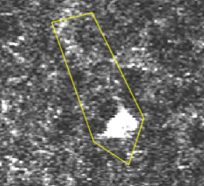
A transient, where several pixels coactivate.

It takes as an input an array of voltage traces, projects them in a 2D plane using t-SNE (\(t\)-distributed Stochastic Neighbor Embedding) [1] and find clusters using HDBSCAN (Hierarchical Density-Based Spatial Clustering of Applications with Noise) [2].

---

Dimensionality reduction

Before clustering the traces, it is important to build a relevant metric in order to assess their proximity. This metric can then be used to compute the distance matrix between the traces, which enables their projection in a 2D space, to simplify the representation and increase the clustering computation speed.

PCA

As t-SNE algorithm needs low dimension inputs to run fast, we first reduce the traces dimensionality using PCA (Principal Components Analysis).

t-SNE

Then we define relevant distance metric to assess traces correlation. In our case, the most famous one is “Pearson correlation” [5], which measures the linear correlation between two variables. “Spearman’s rank correlation” [5] is also particularly adapted in our case. This allows to compute the distance matrix of the components traces, which t-SNE processes to project them into a 2D plane with a non-linear method.

---

Clustering

Once the traces are projected in a 2D plane, we apply HDBSCAN.

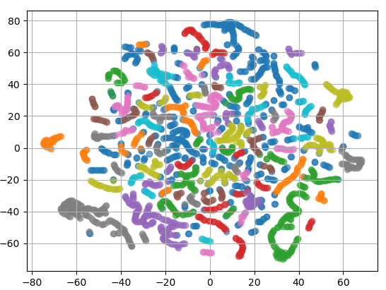
A plot of 2D projected traces.

Each point represents one component. The components having “similar” traces (based on the distance matrix) are close, and the clustering algorithm forms colored groups.

---

Parameter selection

Dimensionality reduction

This parameter section is related to the Dimensionality reduction.

Selecting normalization_method

• type: str
• default: 'z-score'

The normalization_method parameter selects the method for normalizing the traces. The choices are:

• 'null': no normalization
• 'mean-substraction': \(T = T - \overline T\)
• 'z-score': \(T = (T - \overline T) / \sigma(T)\)

Note

The normalization is done again to make sure the dimensionality reduction is under the right format. If the traces were already normalized during skeletonization, there is no need to do it again.

Selecting pca_variance_goal

• type: float
• default: 0.90

The pca_variance_goal parameter selects the percentage of variance to keep after PCA. It must be a float inferior to 1. The higher it is, the more principal components are kept.

Tip

The advantage of setting a percentage goal is that you keep control on the level of information you want to keep on the traces. You can also input an int, if you know the exact number of components you want to give to the following t-SNE algorithm. But be aware of the fact that you might loose a lot of information if you set it too low.

Tip

The effects of this parameter can be seen on the “before/after” graphs by inspecting the dimensionality_reduction/ folder generated when launching the clustering module.

Selecting tsne_distance_metric

• type: str
• default: 'spearman'

The tsne_distance_metric parameter selects the distance metric for t-SNE distance matrix computation. It can be one of pearson, spearman and every metric in sklearn.metrics.pairwise.distance_metrics.

Tip

The effects of this parameter can be directly seen on the clusters plots by inspecting the hdbscan_clustering/ folder generated when launching the clustering module. For instance, the clusters traces found using spearman will be largely different from the ones using euclidean.

Selecting tsne_perplexity

• type: int
• default: 30

The tsne_perplexity parameter selects “the number of nearest neighbors that is used in other manifold learning algorithms” [1].

Important

The value needs to take into account the typical size of clusters we want. For instance, if we want to cluster skeleton pixel components, the perplexity needs to be much higher than if we want to cluster branches. An example is done in Consecutive clusterings.

Tip

The effects of this parameter can be directly seen on the point distribution in the scatter plot by inspecting the hdbscan_clustering/ folder generated when launching the clustering module.

Selecting tsne_random_state

• type: int
• default: 42

The tsne_random_state parameter selects the random number generator for t-SNE algorithm. For reproducible results, pass an int.

---

Clustering

This parameter section is related to the Clustering.

Selecting min_cluster_size

• type: int
• default: 5

The min_cluster_size parameter selects the minimum size of clusters. For more details on how to set this parameter correctly, see [4].

Tip

The effects of this parameter can be directly seen on the colors of the scatter plot by inspecting the hdbscan_clustering/ folder generated when launching the clustering module.

Selecting min_samples

• type: int
• default: 5

The min_samples parameter selects “the number of samples in a neighbourhood for a point to be considered a core point” [3]. For more details on how to well couple this parameter with min_cluster_size, see [4].

Selecting hdbscan_metric

• type: str
• default: 'euclidean'

The hdbscan_metric parameter selects “the metric to use when calculating distance between instances in a feature array” [3].

[1]	(1, 2) t-SNE, Scikit-Learn, https://scikit-learn.org/stable/modules/generated/sklearn.manifold.TSNE.html

[2]	HDBSCAN Documentation, HDBSCAN, https://hdbscan.readthedocs.io/en/latest/

[3]	(1, 2) HDBSCAN API, HDBSCAN, https://hdbscan.readthedocs.io/en/latest/api.html

[4]	(1, 2) HDBSCAN Parameters, HDBSCAN, https://hdbscan.readthedocs.io/en/latest/parameter_selection.html

[5]	(1, 2) Clearly explained: Pearson V/S Spearman Correlation Coefficient, Juhi Ramzai on Medium, https://towardsdatascience.com/clearly-explained-pearson-v-s-spearman-correlation-coefficient-ada2f473b8