Results and computation
Results
Here you can find a detailed list of the content of the results folder of each analysis. You may want to read the OVERVIEW page that corresponds to the analysis you want to launch before reading this section (see Skeleton, Clustering and Factorization).
- Skeleton (page)
sequence_projection/projected_coordinates.npy: a file containing the array of components coordinatesprojected_traces.npy: a file containing the array of components tracesprojected_mask.png: the binary skeleton (or ‘active’) masksummary_image.png: the summary_image generated from the movie
skeleton_mask/: a folder containing all the intermediate images obtained during image skeletonization:0_summary_image.png1_histogram_equalization.png2_smoothing.png3_thresholding.png4_holes_removing.png5_skeletonization.png6_skeleton_cleaning.png7_skeleton_label.png
- Clustering (page)
dimensionality_reduction/pca_res_*.png: a figure of a trace before and after PCA
hdbscan_clustering/cluster_*.png: a figure containing a cluster mask and traceshdbscan_*.png: a scatter plot of traces, projected in a 2D plane
sequence_projection/: the same folder than in skeleton, but whose components are the clusters (see Consecutive clusterings)
- Factorization (page)
skewness/comp_*_to_*.png: each output component of the factorization, before the skewness selection, with a red or green outline depending on whether the skewness is high enough to be kept (green) or not (red)skewness_distribution.png: histogram distribution of the components’ skewnesses
components/comp_*.png: each final component of the analysis
Computational performance
Here are plotted the execution durations of the different modules for some movies. The execution times may vary slightly with the methods and parameters selected. Experiments were conducted on a Intel(R) Core(TM) i7-8565U CPU @1.80GHz.
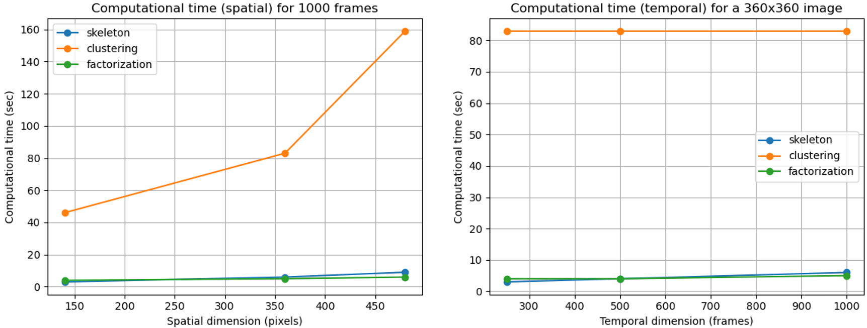
Computational time of the three modules.
Tip
Depending on which operation you want to perform on the sequence, you can adjust some parameters (e.g. crop) to increase computational speed. You can also cut your movie into smaller ones (e.g. \(12500 = 5 \times 2500\) frames).

Cropping process diagram.