Skeleton

In the next sections, the method illustrations (results, inputs…) focus on our study on Calcium Imaging data from the mice hippocampus (see Motivation for more info).

---

Methods

The skeleton module focuses on the morphological analysis of the data. It also reduces the dimensions of it, which is very useful to reduce the computational time of the activity analysis that can be run behind it.

A two-photon calcium imaging movie.

Sequence denoising

First of all, in order to remove the noise from the sequence, we use a 3D gaussian smoothing. It allows to reduce both spatial and temporal noises.

Image skeletonization

Assuming that the movies are well motion corrected and that not too much branches overlap, the filmed stack can be “summed up” with one image, representative of the real physical morphology of the imaged stack. An easy way of doing this is taking the temporal mean image of the movie, but other elementary methods were implemented.

Once we have this summary image, we apply some image processing methods to extract its skeleton. The following paragraphs detail the method used to skeletonize the summary image.

Note

Almost every sub-method is flexible to the input data. Several tips on how to adjust the method parameters are given in the corresponding parameter selection section.

Histogram equalization

As the somata have a very high intensity throughout the movies, we have to be sure that they will not have a significant influence over the binarization method – which is based on a local intensity thresholding. To prevent this from happening, we firstly perform an histogram equalization. This image processing method consists in flattening the distribution of the image intensities in order to enhance the contrast.

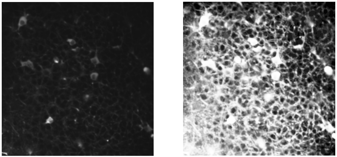
Left: summary image; Right: histogram equalization.

Gaussian smoothing

The image noise can be problematic during the binarization. Indeed, the consequent local intensity fluctuation makes the thresholding algorithm generate small “holes” on the binary structure. In order to limit their presence, we smooth the equalized image with a Gaussian filter.

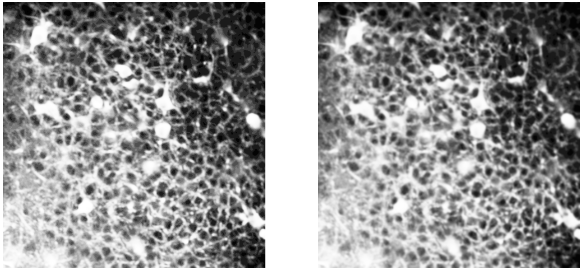
Left: histogram equalization; Right: gaussian smoothing.

Adaptive thresholding

Once the image is well contrasted and smoothed, we binarize it with an adaptive Gaussian thresholding. Contrary to the classic thresholding methods, that set a global threshold for the image intensities, the adaptive thresholding changes the threshold depending on the local environment, which allows it to deal with eventual intensity shifts, like shadows zones for instance. For more details, see [1].

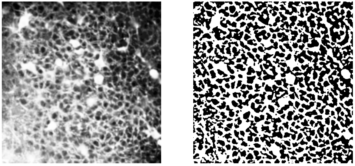
Left: gaussian smoothing; Right: adaptive thresholding.

Holes removing

Even with the preventive Gaussian smoothing, some small “holes” may still remain in the binary skeleton. It is important to get rid of them because they can cause the resulting skeleton to go around them, not only missing the heart of the structure, but also creating useless cycles around the holes. Thus, we developed a simple method that detects the small holes in the binary image and “fills” them.

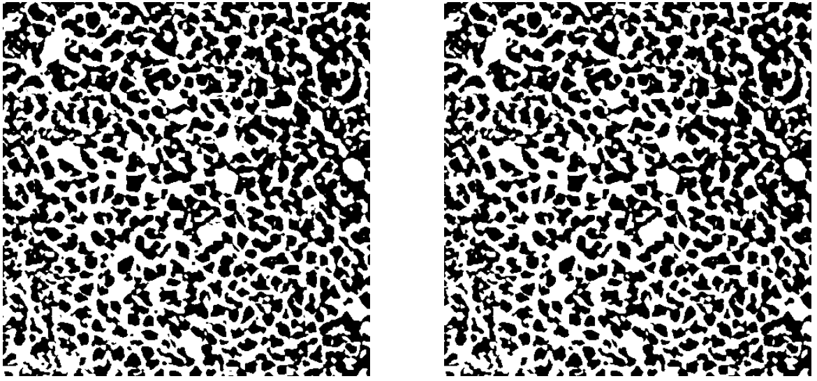
Left: adaptive thresholding; Right: holes removing.

Skeletonization (Lee)

Once the binary structure is clean, we are able to skeletonize it with Lee’s method. For more details, see [2].

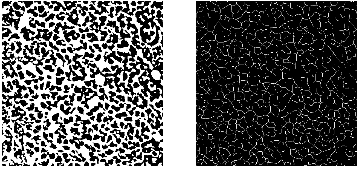
Left: holes removing; Right: skeletonization (Lee).

Parasitic skeletons removal

During skeletonization, the isolated spots in the binary image are converted to small isolated skeletons. They are not harmful, but we can still eliminate them to clean the skeleton structure.

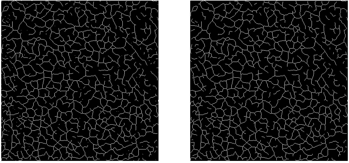
Left: skeletonization (Lee); Right: parasitic skeletons removing.

Results

Finally, we can project the sequence on the computed skeleton and thus reduce its dimensionality.

Intensity projection on the skeleton, pixel by pixel.

Note

This projection, pixel by pixel, is obtained by setting projection_method to 'pixel'. For more details, see Parameter selection.

---

In-depth skeleton analysis

We can get statistics out of the skeleton mask using the python package skan.

By comparing the skeleton structure to a non-oriented graph, this package allows to decompose the skeleton into a set of branches and get some information about them: coordinates of their pixels, lengths, neighbors, etc… By gathering all this data, we can get morphological statistics about the structure of the image and clean it by removing some specific branches. For more details about this package, see [3].

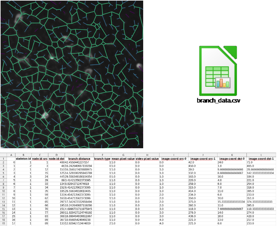
Left: skeleton overlaying; Right: logo .csv file containing branch DataFrame; Bottom: branch DataFrame extract.

As explained in the Motivation section, “there is no obvious correlation between the morphological ‘branches’ that one can see on the videos, and the neurites, that are coactive functional entities”. That is why we are naturally tempted to uniformize the intensity along each branch, to conclude whether the averaging is biologically correct.

Here is an example of sequence projected on branches with intensity uniformization.

Intensity projection on the skeleton, branch by branch.

Note

This projection, branch by branch, is obtained by setting projection_method to 'branch'. For more details, see Parameter selection.

---

Branch uniformity study

To check whether this branch intensity uniformization is legitimate, we drew from Gauthier et al. method [4], and developed transient-by-transient visualization module to classify the morphological branches, in two categories: valid and not valid. A branch is qualified as “valid” if its intensity during its transients is uniform. It confers the branch a functional interpretation, as a part of one and only one neurite, which allows to average its pixels intensities. To quantify the uniformity, we used the skewness metric (see [5]).

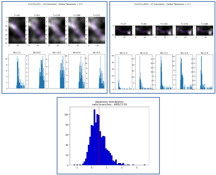
Top: screenshots of the visualization module; Bottom: distribution of skewness among the branches.

Depending on the movie, the number of remaining branches may vary.

Intensity projection on the valid branches.

---

Parameter selection

Sequence denoising

Here are the parameters that affect the sequence denoising.

Tip

The effects of these parameters can be seen by setting the parameter save_denoised_sequence to True and inspecting the preprocessing/ folder generated when launching the skeleton module.

Selecting denoising_method

• type: str
• default: '3D'

Method used to denoise the sequence. The choices are:

• '2D': Smooth each frame;
• '3D': Smooth the whole sequence, as a 3D image.

Selecting sigma_denoising

• type: float
• default: 1.0

Sigma in gaussian smoothing for denoising the sequence.

Warning

When denoising_method is set to '3D', the smoothing is also temporal. In order to keep the transients locality, you must be careful of not setting it too high.

Image skeletonization

Here are the parameters used to perform Image skeletonization.

Tip

The effects of these parameters can be seen individually on the intermediate images by inspecting the skeleton_mask/ folder generated when launching the skeleton module.

Important

These parameters are essentially morphological. Thus they need to be adapted to the scale and resolution of the input sequence. You might need several tests to find good parameter values.

Selecting summary_method

• type: str
• default: 'mean'

The summary_method parameter selects which method to use for the generation of a summary image from the .tif movie. The choices are:

• 'mean': get the mean image along the time axis.
• 'median': get the median image along the time axis.
• 'standard_deviation': get the standard deviation image along the time axis.

Note

When summary_method is set to 'standard_deviation', it is needed to group some frames before computing the sequence standard deviation. That is the role of the next parameter, std_grouping_ratio.

Selecting std_grouping_ratio

• type: int
• default: 10

The std_grouping_ratio parameter selects the number of sequence frames to group and average before computing the sequence standard deviation, in order to remove noise from the summary image. It should be large enough to remove the noise, but not too high, in order to preserve the intensity variations of the neurites.

Selecting projection_substructure

• type: str
• default: 'skeleton'

The projection_substructure parameter selects which structure is used for the mask on which we project the intensities.

• 'skeleton': the mask is the skeletonized image.
• 'active': the mask is the binary image, just before the step of skeletonization in Image skeletonization.

The interest of this method is detailed in Skip skeletonization.

Selecting sigma_smoothing

• type: float
• default: 1.0

The sigma_smoothing parameter selects the standard deviation for Gaussian kernel. The higher it is, the smoother is the image, and the fewer holes there are in the binary image.

Selecting adaptive_threshold_block_size

• type: int
• default: 43

The adaptive_threshold_block_size parameter selects the size of a pixel neighborhood that is used to calculate a threshold value for the pixel. It must be odd. For more details, see [1].

Tip

Should be set so that the block captures a soma + a bit of its environment. For example, if in the movie a typical soma size is \(30\times 30\) pixels, then 43 should be a good value for adaptive_threshold_block_size to capture the environment.

Selecting holes_max_size

• type: int
• default: 20

The holes_max_size parameter selects the maximum size (number of pixels) of the holes we want to fill in the binary image. As explained in Image skeletonization, some parasitic holes may appear during binarization. Most of the time, they appear inside the somas or inside the branches, due to defects in thresholding.

Important

These parasitic holes must not be confused with larger holes, representing rings, or simply void between branches.

Tip

A good advice to find the perfect value, is to identify the minimum size of the holes we want to keep (small rings for instance), and take a threshold just below.

Note

To remove the objects, we use the scikit-image method remove_small_objects, with connectivity=1, which means that two diagonal black pixels are not considered as part of the same hole. For more details, see [6].

Selecting parasitic_skeletons_size

• type: int
• default: 5

The parasitic_skeletons_size parameter selects the maximum size (number of pixels) of isolated skeletons (see Image skeletonization) we want to remove.

Note

To remove the objects, we also used the scikit-image method remove_small_objects, but this time with connectivity=2, which means that two diagonal white pixels are considered as part of the same skeleton.

---

Projection method

As explained in Image skeletonization, two components are analyzed in our trace study: pixels of the skeleton individually, and branches of the skeleton. Respectively, two projection methods are developed: pixel and branch.

Selecting projection_method

• type: str
• default: 'pixel'

The projection_method parameter selects the projection method. For pixels, we simply take the coordinates of the white pixels, and get their trace. For branch, we first get the coordinates of all the pixels in the branches, using the skan package, and then average their intensity, through time.

---

Trace processing

This parameter section is related to the various signal processing methods used to clean the traces.

Selecting element_normalization_method

• type: str
• default: 'z-score'

The element_normalization_method parameter selects the method for normalizing the traces. The choices are:

• 'null': no normalization
• 'mean-substraction': \(T = T - \overline T\)
• 'z-score': \(T = (T - \overline T) / \sigma(T)\)

Note

The common method for trace processing is z-score, because it allows to set en the same footing all the elements we consider. But we can imagine some cases where this method is not suitable, for instance if we want to give more importance to the somatas, which have high intensities.

Selecting element_smoothing_window_len

• type: int
• default: 11

The element_smoothing_window_len parameter selects the dimension of the smoothing window used for convolution. It must be odd.

Warning

Set it below the minimum frame difference between two transients. Otherwise, 2 transients would be merged !

Selecting branch_radius

• type: int
• default: 1

The branch_radius parameter selects the radius of the branches.

Note

In the case of pixel, it is only for display, but in the case of branch, all the pixels in the dilated branch are taken into account in the branch intensity averaging.

---

Branch validation

This parameter section is related to the Branch uniformity study.

Selecting pixels_around

• type: int
• default: 5

The pixels_around parameter selects the number of pixels to display around the analyzed branch, for visualization. See Branch uniformity study for an example.

Selecting peak_properties

• type: dict
• default: height=None, threshold=None, distance=None, prominence=3, width=None

The peak_properties parameter selects the properties relative to the trace peaks, in order to consider an activity variation as a transient. It contains different sub-parameters:

• height: required height of peaks.
• threshold: required threshold of peaks, the vertical distance to its neighboring samples.
• distance: required minimal horizontal distance in samples between neighbouring peaks.
• prominence: required prominence of peaks.
• width: required width of peaks in samples.

(Source: scipy find_peaks [7]). For an example on the influence of each parameter, see [8].

Note

The values need to take into account the normalization method. The advantage of z-scoring is that these parameters can be kept for different inputs.

Selecting transient_neighborhood

• type: int
• default: 2

The transient_neighborhood parameter selects the number of frames between the transients onsets and peaks.

Disclaimer

The assumption that the number of frames between transients onsets and peaks is constant is false. However we decided to keep it simple as is doesn’t skew the method’s results. But we could consider to implement a method that automatically detects the transients onsets and offsets, using Scipy’s find_peaks function.

Selecting skewness_threshold

• type: float
• default: 0.5

The skewness_threshold parameter selects the skewness value above which a branch isn’t considered as valid. For more details refer to Branch uniformity study.

[1]	(1, 2) Image Thresholding, OpenCV, https://opencv-python-tutroals.readthedocs.io/en/latest/py_tutorials/py_imgproc/py_thresholding/py_thresholding.html

[2]	Skeletonize, Scikit-Image, https://scikit-image.org/docs/dev/auto_examples/edges/plot_skeleton.html

[3]	Skan’s documentation, Skan, https://jni.github.io/skan/index.html

[4]	“Detecting and Correcting False Transients in Calcium Imaging”, Gauthier et al., https://www.biorxiv.org/content/10.1101/473470v1

[5]	Skewness, Wikipedia, https://en.wikipedia.org/wiki/Skewness

[6]	Remove small objects Scikit-Image, https://scikit-image.org/docs/dev/api/skimage.morphology.html#skimage.morphology.remove_small_objects

[7]	Find peaks Scipy, https://docs.scipy.org/doc/scipy/reference/generated/scipy.signal.find_peaks.html

[8]	Peak-finding algorithm for Python/SciPy stack overflow, https://stackoverflow.com/questions/1713335/peak-finding-algorithm-for-python-scipy